Central Limit Theorem
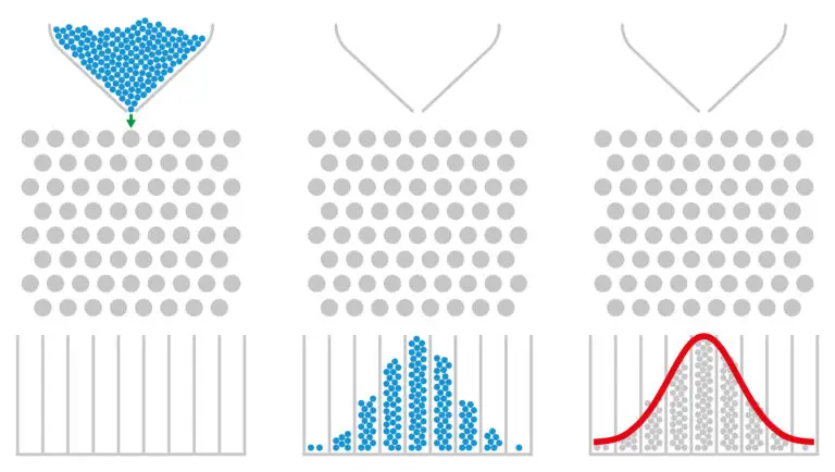
Table of Contents
What is the Central Limit Theorem?
The Central Limit Theorem (CLT) is a fundamental concept in statistics that describes the behavior of the sampling distribution of the sample mean (or sum) as the sample size increases, regardless of the shape of the population distribution.
Assumptions
The Central Limit Theorem (CLT) is foundational in statistics and relies on several key assumptions for its application. Firstly, it assumes that the samples are randomly drawn from the population, ensuring that each sample is representative and unbiased.
Secondly, it posits that each sample is independent of the others, meaning the selection of one sample does not affect the selection of another. This independence is crucial for preventing correlation between samples that could skew the results.
Lastly, the CLT assumes that the sample size is sufficiently large, often suggesting a minimum size of n ≥ 30 to approximate a normal distribution, especially for populations with unknown distributions. However, for populations with a distribution that is not extremely skewed or kurtotic, smaller sample sizes can still lead to a fairly accurate application of the CLT.
Sampling Distribution
The Central Limit Theorem states that the sampling distribution of the sample mean (or sum) will be approximately normally distributed, regardless of the shape of the population distribution, as long as the sample size is large enough.
Mean and Standard Deviation
The mean of the sampling distribution of the sample mean is equal to the population mean (μ). This relationship indicates that the average of the sample means will converge to the population mean as the number of samples increases, reflecting the accuracy of the sample mean as an estimator of the population mean.
The standard deviation of the sampling distribution, commonly referred to as the standard error, is calculated by dividing the population standard deviation (σ) by the square root of the sample size (n). Mathematically, this is represented as \sigma / \sqrt{n}. The standard error measures the dispersion of the sample means around the population mean and decreases as the sample size increases. This decrease in standard error with larger sample sizes indicates that the sample mean becomes a more precise estimator of the population mean, reflecting the principles of the Central Limit Theorem.
Normal Approximation
For large sample sizes, the sampling distribution of the sample mean can be approximated by a normal distribution, even if the population distribution is not normal. This allows for the use of normal-based statistical inference methods such as z-tests and confidence intervals.
Applications
The Central Limit Theorem is widely used in hypothesis testing, confidence interval estimation, and other statistical analyses. It allows researchers to make inferences about population parameters based on sample data.
Central Role
The Central Limit Theorem is central to the field of statistics because it provides a basis for generalizing from sample data to the population and for conducting parametric statistical tests even when population distributions are unknown or non-normal.
Example
Let’s consider a scenario where we have a population of IQ scores of all students in a school. The population distribution may not be normally distributed, meaning it might not follow a bell curve.
Now, suppose we take multiple random samples from this population, each containing 50 IQ scores. We calculate the mean IQ score for each sample. According to the Central Limit Theorem, as the sample size increases, the distribution of sample means will approach a normal distribution regardless of the shape of the population distribution.
For example, let’s say we take 100 random samples of 50 IQ scores each from our population. We calculate the mean IQ score for each sample and plot a histogram of these sample means. As we increase the number of samples, the histogram of sample means will start to resemble a bell curve, even if the original population distribution was not normal.
This demonstrates the Central Limit Theorem’s principle that the sampling distribution of the sample mean becomes approximately normal as the sample size increases, regardless of the shape of the population distribution.
Related Links
Bias
Cluster Random Sample
Population
Snowball Sampling